Approximate nearest neighbour search using HSNW
Why K-Nearest Neigbours sucks?
K-Nearest Neigbours(KNN) struggles with scalability. It performs effectively when dealing with small datasets and lower dimensional vectors. However, when it comes to large datasets, a more efficient method for managing data and searching is required. ![]()
Recently, the use of Approximate Nearest Neighbors algorithms has become increasingly important in various vector databases such as Pinecone and weaviate. These databases are utilized for Retrieval-Augmented Generation (RAGs), which involves high-dimensional vector search with millions of records. ![]()

In this post, we’re going to take a look at how to use approximate nearest neighbor search with a graph-based approach. But before we dive into the details, let’s first discuss some key properties of graphs that are super helpful in building this kind of algorithm. ![]()
Properties of a graph
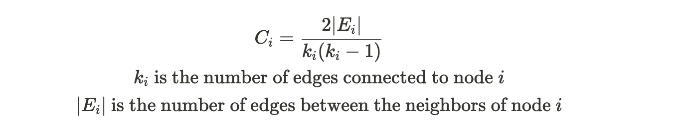
The clustering coefficient
It measures how likely the two nodes connected are part of a larger group in the graph. The cluster coefficient measures the density of connections among nodes in a network, indicating how close its neighbors are to being a complete network themselves. A higher cluster coefficient suggests that nodes tend to form clusters. It can be defined as follows:
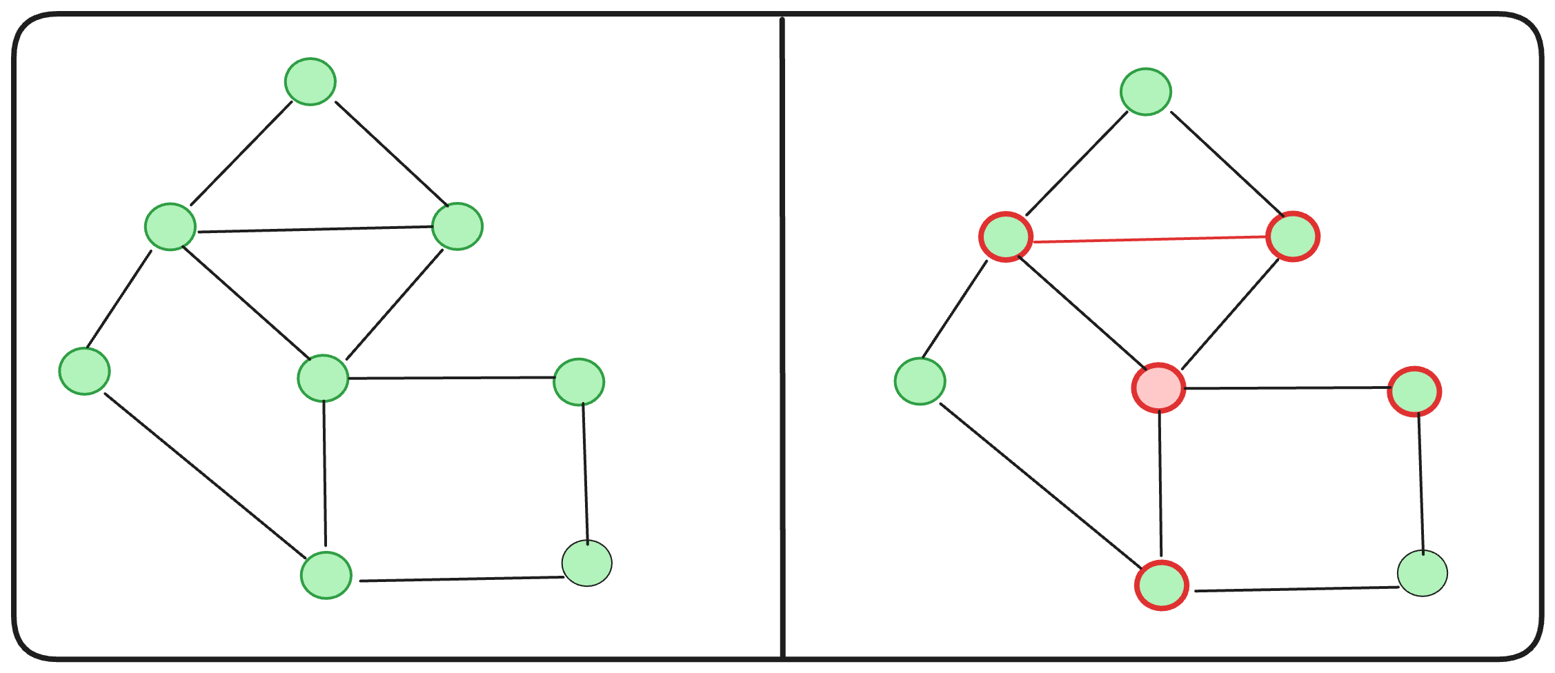
Let’s compute the clustering coefficient of the red node on the graph given.
The graph diameter
It is the shortest distance between the two furthermost nodes in the graph. Ideally, for efficient traversal of nodes, it is recommended that graphs have as small a diameter as possible.
For the figure above, the graph diameter is 6.
What about the cluster-coefficient? C(2) = (2 * 2) / ( 4 * 3 ) = 1/3
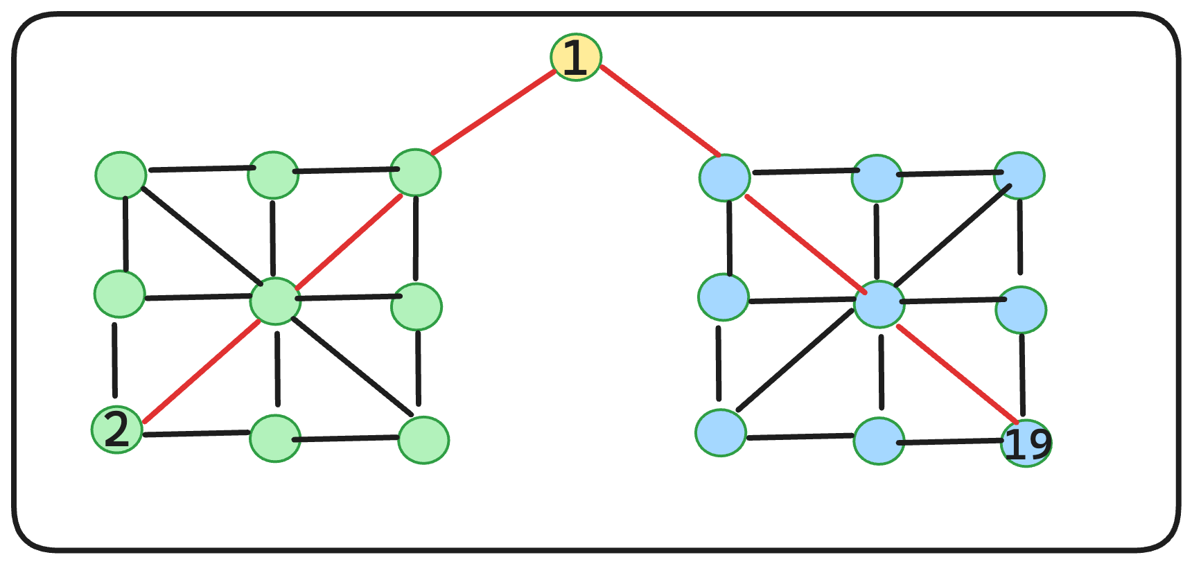
Is it possible to reduce the total diameter of this graph? Absolutely. By introducing an additional edge, as illustrated, we achieve a diameter of 5.
However, how does it affect the cluster co-efficient of the node(2)?
C(2) = ( 2 * 2 ) / ( 5 * 4 ) = 1/5
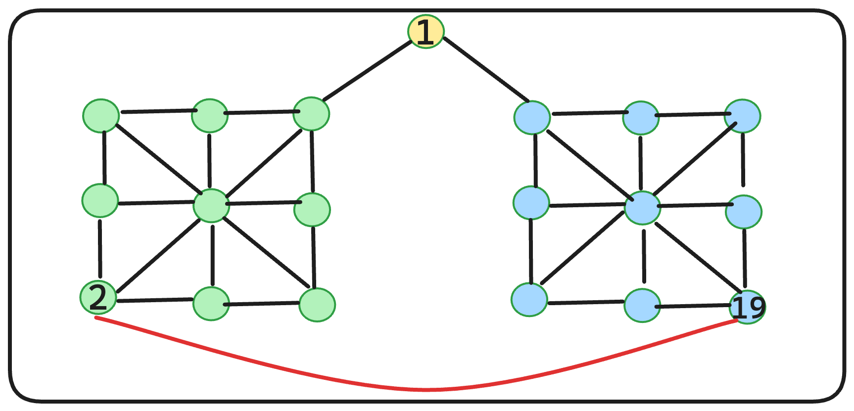
Hmm… adding an extra edge indeed decreases the overall diameter, but it also diminishes the clustering coefficients. We aim for graphs with high clustering coefficients and low diameters to efficiently run computational algorithms. However, as we’ve observed, achieving this balance can be quite challenging. ![]()
Here’s the next query: Is it possible to adjust edges to maintain the clustering coefficient while diminishing the overall diameter? Enter the Navigable Small World algorithm. And fear not, the algorithm is simpler than you might imagine! ![]()
Navigable Small World (NSW) 
Building a Navigable Small World involves removal and addition of edges strategically to the graph, ensuring the clustering coefficient remains intact while reducing the overall diameter. The idea comes from a concept called the “six degrees of separation”, that anyone in the world can be connected to anyone else through a chain of six or fewer people they know. This concept is used to find short paths between any two people or things in a network, like your social media friends or websites on the internet. It’s a pretty cool idea that’s used in a lot of different ways. ![]()
How can we construct a navigable small world?
Within the graph, we traverse each edge. With a probability ( P ), we introduce a random edge between any two nodes within the graph while removing the existing edge. Subsequently, we plot the diameter and cluster coefficient across various ( P ) values. Our selection criteria focus on worlds with small diameters and high cluster coefficients. It’s quite straightforward, isn’t it?
Now, let’s see this in action. Initially, we’ll construct a connected graph.
import networkx as nx
import matplotlib.pyplot as plt

def get_graph(num_nodes):
    # Create a graph
    G = nx.Graph()

    # Add nodes
    for i in range(num_nodes):
        G.add_node(i)

    # Define the pattern for connecting non-consecutive nodes
    non_consecutive_pattern = 2

    # Add non-consecutive edges
    edges_non_consecutive = [(i, (i + non_consecutive_pattern) % num_nodes) for i in range(num_nodes)]
    G.add_edges_from(edges_non_consecutive)

    # Add consecutive edges
    edges_consecutive = [(i, (i + 1) % num_nodes) for i in range(num_nodes)]
    G.add_edges_from(edges_consecutive)

    return G

G = get_graph(100)
# Create a radial layout
pos = nx.spiral_layout(G)
# Draw the graph
nx.draw(G, pos, with_labels=True, node_color='skyblue', node_size=40, edge_color='gray', linewidths=1, font_size=10)
# Show the plot
plt.show()
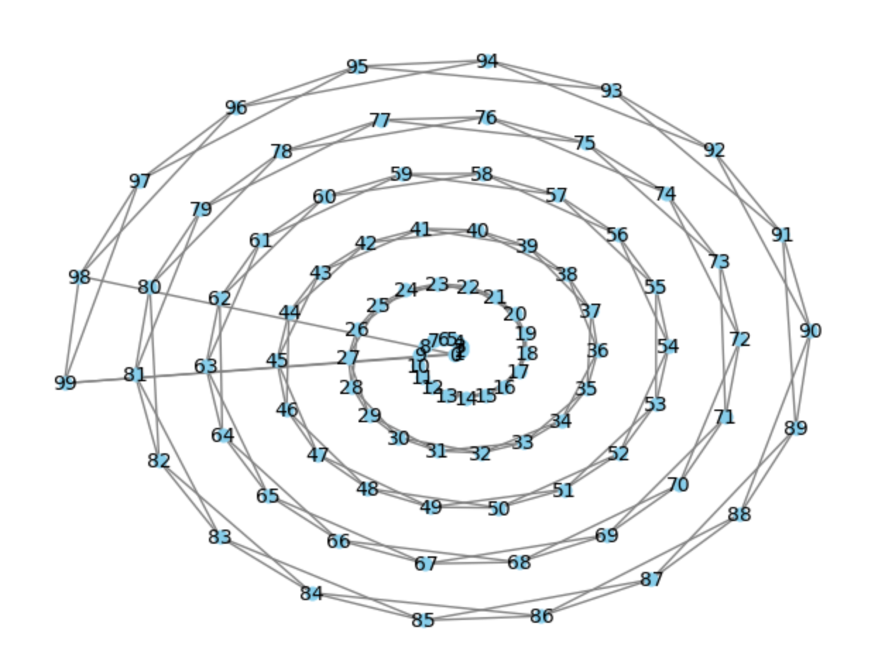
Compute the diameter and clustering coefficient for graph ( G ).
Diameter of the graph: 25
Clustering coefficient of the graph: 0.5
As you can see, the graph has a pretty high diameter overall.
Now, let’s put the NSW algorithm to test.
import networkx as nx
import numpy as np

# Define probabilities from 0 to 1 with gap 0.01
probabilities = np.arange(0, 1.01, 0.01)

# Dictionary to store results
results = {'p': [], 'diameter': [], 'clustering_coefficient': []}

# Iterate over probabilities
for p in probabilities:
    G = get_graph(100)
    all_nodes = set(G)
    for u, v in G.edges():
        if np.random.random() < p:
            u_neighbours = set([u]) | set(G[u])
            new_nodes = all_nodes - u_neighbours
            v_random = np.random.choice(list(new_nodes))
            # Delete the edge
            G.remove_edge(u, v)
            if not nx.is_connected(G):
                G.add_edge(u, v)
            # Add random edge
            G.add_edge(u, v_random)

    # Calculate diameter and clustering coefficient
    diameter = nx.diameter(G)
    clustering_coefficient = nx.average_clustering(G)

    # Store results
    results['p'].append(p)
    results['diameter'].append(diameter)
    results['clustering_coefficient'].append(clustering_coefficient)

# Print results
for i in range(len(probabilities)):
print(f"p={results['p'][i]:.2f}, Diameter={results['diameter'][i]}, Clustering Coefficient={results['clustering_coefficient'][i]:.4f}")p=0.00, Diameter=25, Clustering Coefficient=0.5000
p=0.01, Diameter=22, Clustering Coefficient=0.4873
p=0.02, Diameter=14, Clustering Coefficient=0.4720
p=0.03, Diameter=20, Clustering Coefficient=0.4757
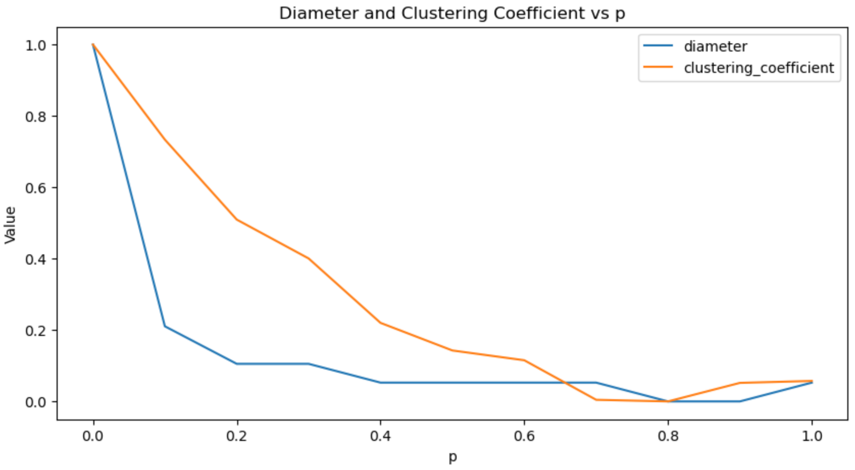
...At ( p = 0.02 ), we observe a 44% reduction in diameter with only a 2% decrease in the clustering coefficient. Plotting the normalized scores, we notice that beyond a certain threshold, higher probabilities result in lower diameters and clustering coefficients ![]() .
.
Hierarchical Navigable Small World (HNSW) 


HNSW extends the concept of NSW (Navigable Small World) by introducing multiple layers stacked atop one another. Each node may exist on a subset or all of the defined layers. The determination of a node’s occurrence on a layer is computed using the formula:
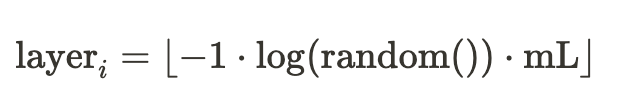
The hyperparamer mL is used to control the level of node insertion.
For example, if we have a total of 10 nodes and define an HSNW (Hierarchical Navigable Small World) with 4 layers, let’s say for node 8, if the layer_i value is 2, then the node will only appear in layers 1 to 2. While every node is present in layer 1, there’s no guarantee they will appear in layers 2 to 4. Additionally, as the value of i increases, the layers become less dense. Once we allocate the node to each layer, we establish connections between the node and others within the layer based on their distance. The aim is to minimize connections to maintain NSW properties.
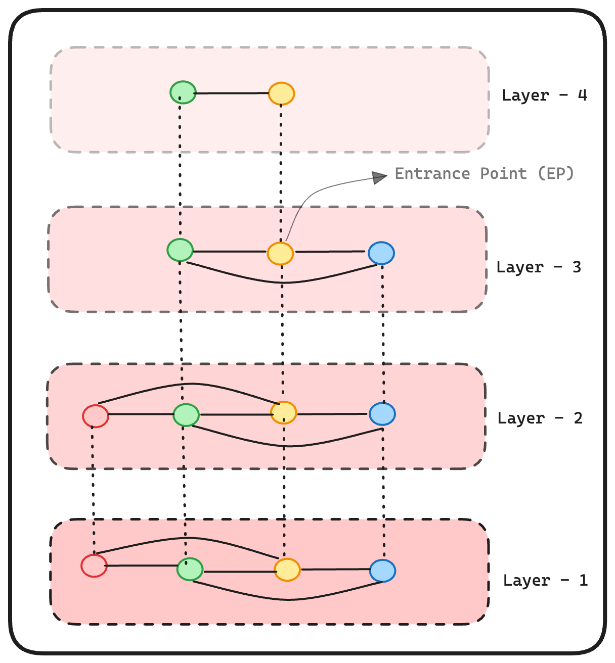
Entrance Points: For the time being, consider entrance points as nodes that facilitate traversal through the layers in HNSW. I’ll elaborate on how these help us shortly.
So, let’s dive into how the nearest neighbor search operates with HSNW. Imagine we’re in a world filled with cheese, wine, and fruits to munch on. And hey, no need to stress—we’ve got 30 types of cheese ![]() , 30 types of wine
, 30 types of wine ![]() , and a whopping 40 varieties of fruits
, and a whopping 40 varieties of fruits ![]() . Each of these is represented with a 1-dimensional embedding vector, like so:
. Each of these is represented with a 1-dimensional embedding vector, like so:
{
    "Cheese-0":  [0],
    "Cheese-1": [1],
    "Cheese-29": [29],
    "Wine-30":  [30],
    "Wine-31": [31],
    "Wine-59": [59],
    "Fruit-60": [60],
    "Fruit-99": [99],
    ...
}
Now, let’s implement this world.
import networkx as nx
from math import floor, log
from random import random
from scipy.spatial import distance

cheese_nodes = { f"Cheese-{i}": i for i in range(30) }
wine_nodes = { f"Wine-{i}": i for i in range(30, 60) }
fruit_nodes = { f"Fruit-{i}": i for i in range(60, 100) }
all_nodes = { **cheese_nodes, **wine_nodes, **fruit_nodes }
We just created a dataset of all our food items.
Let’s create an empty HNSW graph with 5 layers.
num_layers = 5
HNSW = [nx.Graph() for i in range(num_layers)]
Node insertion in HNSW
def insert_nodes(all_nodes):
    # Iterate through all nodes in the dataset
    for node in all_nodes:
        # Extract the feature vector for the current node
        node_feature = all_nodes[node]

        # Determine the number of layers the node should be added to
        node_layers = floor(-1 * log(random()) * num_layers)

        # Loop through each layer the node should be added to
        for layer_index in range(0, max(min(node_layers, len(HNSW)),1)):
            # Add the node to the current layer of the HNSW graph
            HNSW[layer_index].add_node(node)

            # Get the list of current nodes in the layer
            neighbours = list(HNSW[layer_index].nodes)

            # Calculate the Euclidean distance between the current node and all other nodes in the layer
            nearest_neighbours = [(distance.euclidean([node_feature], [all_nodes[neighbour]]), neighbour) for neighbour in neighbours]

            # Sort the distances in ascending order
            nearest_neighbours.sort(key=lambda x: x[0])

            # Connect the current node to its 5 nearest neighbours in the layer, excluding itself
            for neighbour in nearest_neighbours[:5]:
                if node!=neighbour[1]:
                    HNSW[layer_index].add_edge(node, neighbour[1])

# Insert all nodes into the HNSW graph
insert_nodes(all_nodes)
You have the option to enhance node insertion using various techniques. Additionally, the authors introduce a metric for reducing connections when a node’s degree surpasses a specific threshold to maintain the “NSW” property. However, for the purposes of this post, we assume adherence to the “NSW” property.
You can now check the number of nodes are inserted in each layer of HNSW.
for i in range(num_layers):
print(f"layer-{i} | Total nodes:", len(HNSW[i].nodes))layer-0 | Total nodes: 100
layer-1 | Total nodes: 70
layer-2 | Total nodes: 61
layer-3 | Total nodes: 49
layer-4 | Total nodes: 41As observed, in layer-0, all nodes are present, but as the layer ID increases, the number of nodes decreases, resulting in a significantly less dense graph. This aligns well with our requirements.
Node Search in HNSW
Imagine you’ve got a query and you’re on the hunt for neighbors for a food class that you’re not familiar with, but you’ve got its embedding handy [55.5]. Now, with traditional KNN, you’d have to calculate the distance between your query [55.5] and every single sample in the training set. But that’s not the route we want to take!
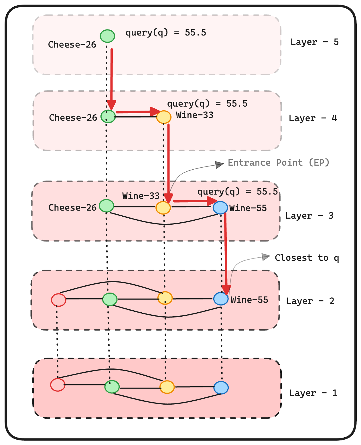
The idea is to start from the layer with the least number of nodes, then find the node that is closest to the query vector. Then this node becomes the entrance point to the next layer. Then, you go to the next layer and search around the neighbours of the entrance point node. If you find a node that is closer to the query vector than the current entrance point, then you make this node a new entrance point to the next layer. The search ends when you do not have any further nodes to explore. But, there are a lot of optimizations that are possible here, we do not implement them here.
So, in our scenario, the query vector [55.5] is initially compared with Cheese-26 in layer-4. As Cheese-26 lacks any neighbors, it serves as the entry point for layer-3. Upon inspecting the neighbors of Cheese-26 in layer-3, we encounter Wine-33. Since Wine-33 is closer (as determined by computing the Euclidean distance) to the query vector [55.5] than Cheese-26, Wine-33 becomes the new entry point for layer-2 as it also lacks neighbors. This process is repeated layer by layer until we arrive at Wine-55, which is the closest to the query vector [55.5]. The search ends at this point.
Here is the graphical representation of this algorithm:
I use Euclidean distance for distance calculation because I’m working with a one-dimensional vector. However, you have the option to use cosine similarity instead.
def compute_distance(q, neighbours):
    # Calculate the Euclidean distance between the query point and each neighbor
    nearest_neighbours = [(distance.euclidean([q], [all_nodes[neighbour]]), neighbour) for neighbour in neighbours]

    # Sort the neighbours by distance in ascending order
    nearest_neighbours.sort(key=lambda x: x[0])

    # Return the index of the closest neighbour
    ep = nearest_neighbours[0][1]
    return ep

def search_nodes(q):
    # Initialize the entry point as None
    ep = None
    # Start the search from the highest layer of the HNSW graph
    for i in range(len(HNSW)-1, -1, -1):
        layer = HNSW[i]
        # If the entrance point is None, compute the distance between the query point and all nodes in the layer
        if ep is None:
            ep = compute_distance(q, layer)
        # Otherwise, compute the distance between the query point and the neighbours of the current entrance point in the layer
        else:
            try:
                neighbours = layer.neighbors(ep)
                ep = compute_distance(q, neighbours)
            except Exception as e:
                # If there are no neighbours, return the current entry point
                return ep
    # Return the final entrance point as the result of the search
    return ep
Now, let’s run the search.
search_nodes(55.5)
'Wine-56'
Fantastic, we reach Wine-56 ![]() without needing to search and compare every single node in the dataset! 🙂
without needing to search and compare every single node in the dataset! 🙂
While the outcome might differ slightly due to the nature of “approximate” nearest neighbor search, it should still be fairly close to the result presented here.
References
[1] https://www.youtube.com/watch?v=ZrDpzzVWwFs&t=477s&ab_channel=StanfordOnline